From 351s to 253s — Feature Engineering, Neural Nets, and Why Statistics Beat XGBoost
Zone-pair median -- a dictionary lookup with no machine learning at all -- beats XGBoost by 15%. That one finding shaped everything I built after it. The signal was in the data, not the model.
This is the first of two posts about building an ETA prediction engine for NYC taxi trips. This post covers the feature engineering that provided most of the signal, and four iterations of a neural network that squeezed out the rest. The next post covers the ensemble that broke through the ceiling -- LightGBM, a FT-Transformer built from scratch, and ONNX inference optimization.
Code is on GitHub. Pre-trained models on HuggingFace.
The Problem
Predict how long a NYC taxi trip will take, given four fields: pickup zone, dropoff zone, request timestamp, and passenger count. That's it. 37 million trips from 2023, scored on Mean Absolute Error against a held-out 2024 winter-holiday eval set.
Constraints: inference under 200ms per request on CPU. Docker image under 2.5GB. No external API calls. No 2024 data in training.
The challenge provided an XGBoost baseline at 351 seconds MAE. The question was how far below that I could get.
Feature Engineering: Where the Signal Lives
The raw dataset gives you almost nothing to work with. Four fields. Duration is the target. Everything else has to be built.
The first thing I tried was the simplest possible approach: for every (pickup, dropoff) pair in the training data, compute the median trip duration. At inference time, look it up. No model, no training, just a dictionary.
Result: 296.7 seconds MAE. That beats XGBoost (351s) by 15% with zero machine learning.
This told me two things. First, the dominant signal is the pickup-dropoff pair itself. A trip from zone 236 to zone 237 takes roughly 600 seconds regardless of time, day, or model complexity. Second, everything else -- time of day, neural networks, ensemble methods -- is refinement on top of this foundation.
Bayesian Shrinkage
The naive approach has a problem: sparse pairs. There are 44,697 unique zone pairs in the training data out of 70,225 possible combinations. Many pairs have fewer than 10 trips. Computing a mean from 3 trips gives you noise, not signal.
Bayesian shrinkage fixes this by pulling sparse estimates toward a prior:
smoothed = (n * pair_mean + 20 * zone_mean) / (n + 20)
Where n is the number of trips for that pair, and zone_mean is the average duration for that pickup zone. With 20 as the prior count, a pair with 3 trips gets heavily smoothed toward the zone average. A pair with 10,000 trips is barely affected.
For pairs that don't exist at all in the training data (492 rows in the dev set), there's a fallback hierarchy:
pair-level stats → pickup zone mean → dropoff zone mean → global mean (989s)
This hierarchy ensures every prediction has a reasonable starting point, even for routes the model has never seen.
Time Bucketing
The same zone pair varies 2.2x by time of day. Zone 237 to 236 takes 251 seconds at 5 AM but 552 seconds at 2 PM. A single pair mean collapses this variation into one number.
I split the day into 6 traffic regimes:
| Bucket | Hours | Regime |
|---|---|---|
| 0 | 12 AM - 5 AM | Late night |
| 1 | 5 AM - 8 AM | Early morning |
| 2 | 8 AM - 11 AM | AM rush |
| 3 | 11 AM - 4 PM | Midday |
| 4 | 4 PM - 8 PM | PM rush |
| 5 | 8 PM - 12 AM | Evening |
For each (pickup, dropoff, time_bucket) triplet, I computed Bayesian-smoothed mean and median durations. The temporal prior count is 10 (lighter than the pair-level 20) because splitting by time bucket makes the data sparser.
Time-bucketed pair mean alone scored 277.9s -- a 25-second improvement over the flat pair median, and 21% below the XGBoost baseline. Still no machine learning.
The Full Feature Set
In total, I built 24 continuous features across two groups:
Zone-pair statistics (14 features):
| Feature | What it captures |
|---|---|
pair_mean_smoothed |
Bayesian-shrunk average duration |
pair_median |
Robust central estimate |
pair_std |
Route variability |
pair_p25, pair_p75 |
Duration range bounds |
pair_iqr |
Interquartile range (predictability) |
pair_count |
Raw trip count |
log_pair_count |
Log-scaled count (better for neural nets) |
same_zone |
Binary: pickup == dropoff |
pu_mean, do_mean |
Zone-level averages (fallback signal) |
pair_tb_mean |
Time-bucketed pair mean (shrunk) |
pair_tb_median |
Time-bucketed pair median |
pair_rarity |
1/(1+log1p(count)) -- high for rare pairs |
Temporal features (10 features):
| Feature | What it captures |
|---|---|
hour_sin, hour_cos |
Cyclical hour encoding |
dow_sin, dow_cos |
Cyclical day-of-week |
month_sin, month_cos |
Cyclical month |
minute_of_day |
Normalized [0, 1] |
is_weekend |
Binary flag |
is_rush_hour |
Weekday 7-9 AM or 4-7 PM |
is_night |
11 PM - 5 AM |
Cyclical encoding (sin/cos) matters because hour 23 and hour 0 are one hour apart, but a linear encoding treats them as 23 units apart. The sin/cos pair preserves the circular relationship.
Plus 2 categorical features (pickup zone and dropoff zone IDs) fed directly into embeddings.
Memory-Efficient Processing
One practical detail that took longer than expected: 37 million rows with 24 features doesn't fit in memory on Kaggle's 13GB RAM. The pipeline processes data in 2 million-row chunks, using integer-encoded pair keys (pickup * 1000 + dropoff) instead of tuple objects. Python tuples are 56 bytes each -- switching to integer keys saved 3-4 GB of RAM.
Neural Net v1: Zone Embeddings (272s)
With the features in place, I built a tabular neural network with two branches:
Zone branch: Separate learned embeddings for pickup (266 x 50) and dropoff (266 x 50) zones, plus a hash-based pair embedding (16,384 buckets x 16 dimensions). These get concatenated and processed through a 2-layer MLP.
Continuous branch: The 24 engineered features, batch-normalized, through a separate 2-layer MLP.
Both branches output 128-dimensional vectors that get concatenated (256 total) and processed through a combined MLP with residual blocks down to a single duration prediction.
A few design decisions that mattered:
Separate pickup/dropoff embeddings. The same zone means different things as origin versus destination. Zone 132 (near JFK) as a pickup means someone just landed -- likely heading into Manhattan, 30-60 minute trip. As a dropoff it means someone's going to the airport -- different time of day, different traffic patterns. Shared embeddings would collapse this distinction.
Hash-based pair embedding. Each (pickup, dropoff) pair maps to a bucket via deterministic hashing: (pickup * 7919 + dropoff * 104729) % 16384. This gives the model direct pair-level learning without enumerating all 70K possible combinations. Large primes ensure good mixing. These 262K parameters (47% of the model) turned out to be critical -- reducing to 8K buckets later caused a 13-second regression.
OneCycleLR with warmup. Learning rate warms from 2e-5 to 5e-4 over the first 10% of training, then cosine decays to 5e-7. The warmup is essential -- without it, randomly initialized embeddings produce extreme gradients that cause NaN loss on epoch 1. I learned this the hard way when CosineAnnealingLR without warmup crashed immediately.
Training: Huber loss (delta=300), AdamW (weight_decay=1e-4), batch size 8192, gradient clipping (max_norm=1.0), full 37M training rows.
Score: 272.1s at epoch 4, early stopped at epoch 7.
v2: Time-Bucketed Features + Huber Loss (266s)
Error analysis on v1 revealed systematic underprediction on long trips (-970 seconds bias for trips over 2400 seconds). L1 loss treats all errors equally, but Huber loss with delta=300 applies L2 penalty for errors under 300 seconds (smooth, precise) and L1 for errors above (robust, outlier-resistant). This directly targets the long-trip underprediction.
I also added 5 new features: time-bucketed pair mean and median (the 6 traffic regimes from earlier), pair IQR, log pair count, and a same-zone binary flag. The same-zone flag is a strong signal -- same-zone trips average 450 seconds versus 989 seconds globally.
Score: 266.2s at epoch 5. A 6-second improvement, but the learning curve was flattening.
v3: Residual Blocks + Embedding Interactions (264.5s)
The feature ceiling was hit in v2 -- I wasn't going to extract much more from the 24 features. So I changed the architecture.
Two additions to the zone branch:
Element-wise product (pu * do): If two zones have similar trip patterns (both are Midtown Manhattan zones, for example), their embeddings will be similar, and the element-wise product will be large. This acts as a learned "how related are these zones?" signal.
Element-wise difference (pu - do): A trip from A to B has the opposite sign from B to A. This captures asymmetric effects -- one-way streets, uphill versus downhill, airport arrivals versus departures.
I also added residual blocks in the combined MLP: output = input + MLP(input). These stabilize gradient flow through the deeper network. Each block is Linear → BatchNorm → SiLU → Dropout → Linear.
The model grew from 372K to 560K parameters.
Score: 264.5s at epoch 5. Only 1.7 seconds better than v2. Architecture was hitting diminishing returns.
v4b: Diagnostic-Driven Tuning (264.3s)
Instead of guessing at more architecture changes, I ran deep diagnostics.
Dropout analysis. With dropout at 0.3, the model's predictions had 66 seconds of noise -- the same input produced predictions varying by 66 seconds across random dropout masks. This is excessive regularization. Dropping to 0.15 tightened predictions without increasing overfitting (the train-dev gap stayed at 7.7 seconds, or 3%).
Pair rarity feature. I added pair_rarity = 1 / (1 + log1p(pair_count)), which gives the model an explicit signal for how much to trust the zone-pair statistics. Value of 1.0 for unseen pairs, 0.08 for common pairs. This lets the model learn to weight its own features differently based on data density.
Score: 264.3s. The NN ceiling was confirmed.
The Diagnostic That Changed Everything
I was stuck at 264 seconds. Multiple architecture changes -- deeper networks, wider layers, larger embeddings -- all converged to the same number. Something structural was limiting the model.
I broke down the error by zone-pair frequency:
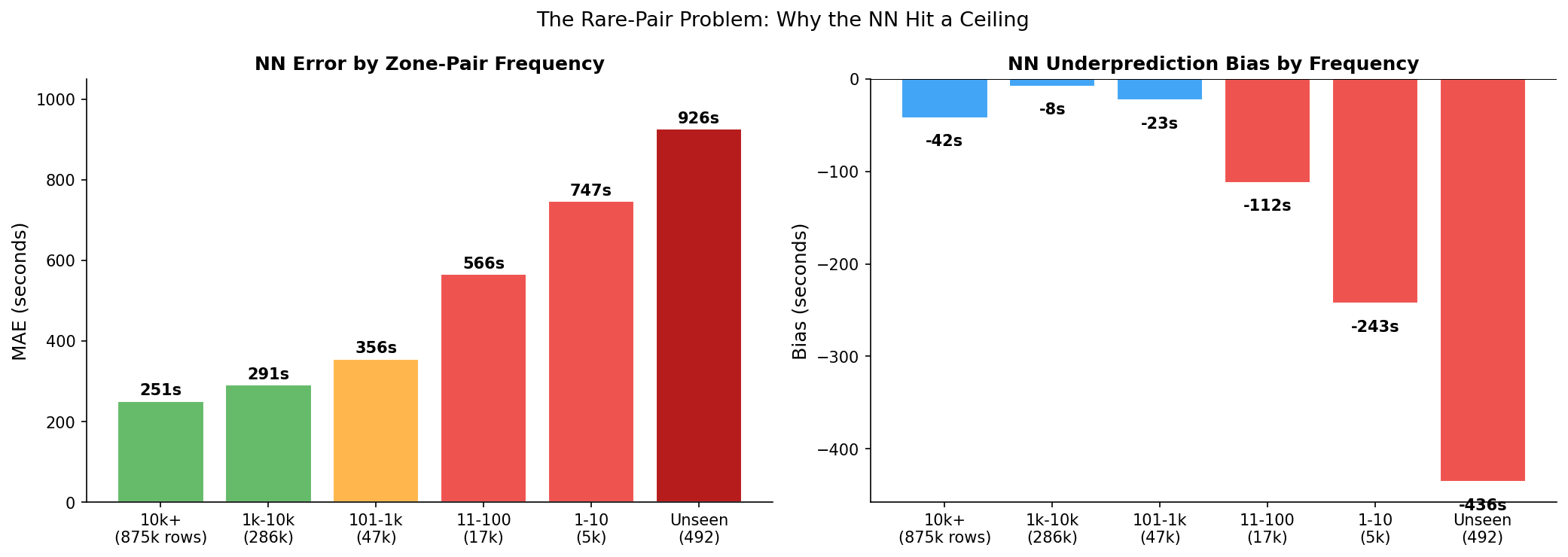
| Pair Frequency | Dev Rows | MAE | Bias | Avg Duration |
|---|---|---|---|---|
| 10k+ trips | 875,471 | 251s | -42s | 849s |
| 1k-10k | 285,659 | 291s | -8s | 1,278s |
| 101-1k | 47,411 | 356s | -23s | 1,524s |
| 11-100 | 16,877 | 566s | -112s | 2,031s |
| 1-10 | 5,001 | 747s | -243s | 2,595s |
| Unseen | 492 | 926s | -436s | 2,829s |
The pattern is clear. For common routes (10K+ trips), the NN is nearly optimal at 251 seconds MAE. But for rare pairs (1-10 trips), error explodes to 747 seconds. For unseen pairs, it's 926 seconds -- catastrophic.
The root cause: neural networks interpolate. Zone embeddings learn representations by averaging over all trips that include each zone. For a rare pair, the embeddings exist (each zone appears in other pairs) but the specific combination has almost no signal. The model defaults to a smoothed average, which systematically underpredicts because rare pairs tend to be long, unusual routes.
No amount of architecture change can fix this. The model needs pair-specific information that doesn't exist in the training data for these routes. A fundamentally different approach was needed -- one that partitions rather than interpolates.
What Didn't Work
Not everything I tried helped. Some experiments made things actively worse:
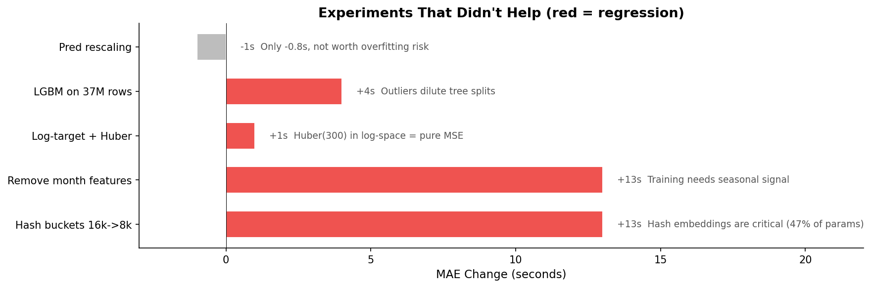
Reducing hash buckets from 16K to 8K. I expected to save 47% of parameters with minimal quality loss. Instead, MAE jumped 13 seconds. At 8K buckets, each bucket averages 5.5 zone pairs instead of 2.8 -- too many collisions. The hash embeddings weren't wasted parameters; they were the most load-bearing component in the model.
Removing month features. The eval set is December. Month features are constant for a single month, so I expected removing them to clean up the signal. Instead, 13-second regression. The training data spans all of 2023 -- the model needs seasonal signal to learn that zone embeddings should account for summer versus winter traffic patterns, even if the eval month is fixed.
Log-target with Huber loss. The duration distribution is right-skewed (median 729s, mean 989s). Training on log-transformed targets should help with skew. But Huber loss with delta=300 in log-space is effectively pure MSE -- log(300) is about 5.7, and almost all log-transformed durations are below that, so the delta threshold never triggers. The loss function wasn't doing what I thought it was doing. Loss-metric mismatch.
Deeper networks past v3. Adding a third residual block, increasing embedding dimensions from 50 to 96, wider hidden layers -- every experiment landed at 264 seconds. The architecture was at its ceiling. More capacity didn't help because the problem wasn't representational power; it was the fundamental limitation of embedding-based interpolation on rare data.
Learning Curves
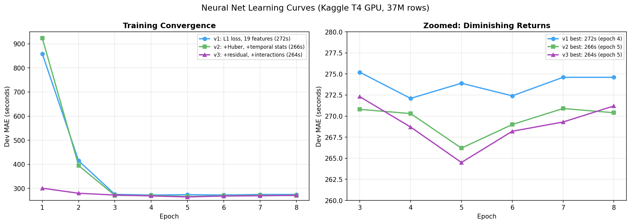
All four versions show the same pattern: rapid convergence in epochs 1-3, best performance around epoch 4-6, then overfitting. Training loss continues to drop while dev MAE rises. The gap narrowed with each version (v1 had 33 seconds gap, v4b had 7.7 seconds), but the shape stayed the same.
The practical lesson: always pick checkpoints by evaluation metric, never by training loss. The model with the lowest training loss is the most overfit model. I checkpoint every epoch and pick the one with the lowest dev MAE.
Where This Stands
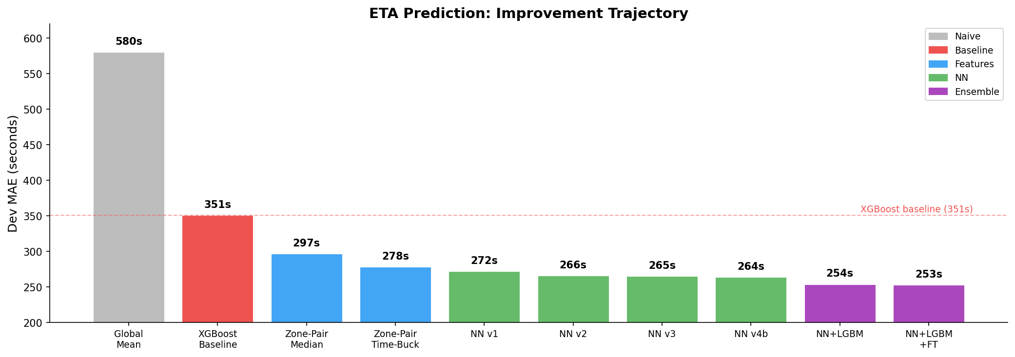
Starting from the 351-second XGBoost baseline:
- Feature engineering alone took it to 278 seconds (zone-pair time-bucketed stats)
- Neural net iterations took it to 264 seconds
- Total improvement: 25% below baseline
But the diagnostic told me the remaining error lives in the long tail -- rare zone pairs where embeddings have nothing to work with. The neural net is near-optimal for common routes. Breaking through 264 requires a model with a completely different inductive bias -- one that doesn't interpolate.
The next post covers that: LightGBM for rare pairs, a FT-Transformer built from scratch, ensemble optimization, and ONNX inference that brought latency from 11ms to 4ms.
Resources
- Code: GitHub
- Pre-trained models: HuggingFace
- Next post: Breaking the NN Ceiling — LightGBM, FT-Transformer, and Ensembles