Breaking the NN Ceiling — LightGBM, FT-Transformer, and Why Ensembles Work
The neural net was stuck at 264 seconds. Four architecture iterations, diagnostic-driven tuning, and nothing moved the needle. The previous post ended with a clear finding: error is dominated by rare zone pairs, and embeddings can't fix what they have no data for.
The fix wasn't a better neural net. It was two completely different models with different failure modes, blended together so their mistakes partially cancel.
Code is on GitHub. Pre-trained models on HuggingFace.
Why Trees Solve What NNs Can't
The neural net's error breakdown told the story: 251s MAE on common routes (10K+ trips), 926s on unseen pairs. The problem is structural. Neural networks learn embeddings by averaging over training examples. For a rare zone pair, the individual zone embeddings exist (each zone appears in other pairs), but the specific combination has almost no signal. The model interpolates between what it knows, and what it knows is "average trip."
Gradient-boosted trees work differently. They don't learn embeddings -- they partition the feature space with hard splits. A tree can learn "if pickup_zone=237 AND dropoff_zone=236, predict 612 seconds" directly, without needing to generalize through a continuous embedding space. Zone IDs are native categorical features, not indices into a learned table.
I trained LightGBM with a straightforward configuration:
objective: mae
num_leaves: 255
learning_rate: 0.05
min_child_samples: 100
feature_fraction: 0.8
bagging_fraction: 0.8
categorical_feature: [pickup_zone, dropoff_zone]
One important finding: 10 million training rows worked better than 37 million. On the full dataset, LightGBM built 138-640 trees and scored 267-274s. On a 10M subsample, it built 81 trees and scored 263s. The theory: outlier trips in the full dataset dilute tree splits, making the learned rules noisier. The tree finds cleaner partitions on cleaner data.
Result: 263.1s MAE with a bias of just -6.3 seconds. Compare that to the NN's -106 seconds of bias. The NN systematically underpredicts because it interpolates rare pairs toward the mean. LightGBM doesn't interpolate -- it either has a specific rule for that zone pair or it doesn't.
The top features by gain: pair_mean_smoothed, dropoff_zone, pickup_zone, pair_median, pair_std. Zone IDs are in the top 3 -- the tree is directly learning zone-level patterns that the NN handles through embeddings.
FT-Transformer: Attention Over Features
The neural net has a hand-designed architecture: separate branches for zones and continuous features, explicit embedding interactions (product and difference), residual blocks in the combined MLP. Every interaction between features was something I decided to include.
What if the model could discover feature interactions on its own?
The Feature Tokenizer Transformer (FT-Transformer) from Gorishniy et al., NeurIPS 2021 does exactly this. The idea: treat each feature as a token -- the same way a language model treats each word as a token -- and let self-attention discover which features should interact.
I implemented it from scratch. Here's how it works:
Step 1: Tokenize Each Feature
Every feature gets projected into a 96-dimensional token through its own independent linear layer:
pair_mean_smoothed (value: 1964) → W_0 * 1964 + b_0 → [96-dim vector]
pair_median (value: 1746)        → W_1 * 1746 + b_1 → [96-dim vector]
is_night (value: 0)              → W_8 * 0 + b_8    → [96-dim vector]
Each feature gets its own W and b. This is critical -- pair_mean_smoothed operates at a scale of ~1000 seconds while is_night is 0 or 1. Shared projections would force them into the same scale. Per-feature projections let each feature learn its own mapping into the token space.
Categorical features (pickup and dropoff zone IDs) go through embedding tables instead: Embedding(266, 96) for each zone.
A learnable [CLS] token is prepended -- it has no input feature, it just aggregates information from all the others.
Result: 27 tokens x 96 dimensions (24 numerical + 2 categorical + 1 CLS).
Step 2: Self-Attention
The tokens pass through 2 transformer encoder layers, each with 4 attention heads (24 dimensions per head), pre-norm architecture (LayerNorm before attention, not after), and a feed-forward network.
What does the attention learn? I can't see the attention weights directly, but the architecture makes certain interactions natural:
pickup_zoneattends todropoff_zone-- route identitypair_rarityattends topair_mean-- how much to trust the statisticshour_sinattends topair_tb_mean-- time-of-day adjustment
The model discovers these interactions from the data. I didn't specify them -- unlike the NN where I explicitly computed pu * do and pu - do.
Step 3: Predict
After 2 layers of attention, the [CLS] token has aggregated signal from all 26 features. It passes through LayerNorm → Linear(96, 1) to produce the duration prediction.
Training
I trained on 10 million rows (same subsample as LightGBM) with L1 loss -- directly optimizing MAE rather than Huber. L1 is simpler and produces cleaner gradients for the attention mechanism. AdamW with lr=3e-4, weight_decay=1e-5, batch size 2048, OneCycleLR with warmup.
Best checkpoint at epoch 5: 267s MAE standalone.
Architecture Compression
The original FT-Transformer from the paper uses d_token=128, 3 layers, 8 heads -- 406K parameters, scoring 287s. I compressed it:
| Dimension | Original | Optimized | Savings |
|---|---|---|---|
| d_token | 128 | 96 | -25% (attention is O(d^2)) |
| Layers | 3 | 2 | -33% compute |
| Heads | 8 | 4 | Richer per-head (24-dim vs 16-dim) |
| FFN multiplier | 4/3 | 1.0 | -44% FFN parameters |
| Total params | 406K | 169K | -58% |
The surprising result: the smaller model scored 267s versus the larger model's 287s. Actually better. With 10M training rows, the 406K parameter model was overfitting -- 2 layers with 169K parameters learned the same patterns without memorizing noise.
This matters for inference too. Fewer parameters means less computation, which becomes important when you need to serve predictions in under 200ms.
Why Ensembles Work
Each model makes different mistakes. That's the entire point of ensembling -- if models made the same mistakes, averaging their predictions wouldn't help.
| Model | Dev MAE | Bias | What it does well | Where it fails |
|---|---|---|---|---|
| NN | 261.2s | -106s | Smooth interpolation for common routes | Underpredicts rare/long trips |
| LightGBM | 261.7s | -6s | Hard partitions on zone IDs, rare pairs | Less precise on common routes |
| FT-Transformer | 267.0s | -1s | Cross-feature attention, fresh error pattern | Weaker standalone |
The NN is the best single model (261.2s) but has a massive -106 second bias. It systematically underpredicts because embeddings smooth rare pairs toward the mean. LightGBM has nearly zero bias (-6s) because trees partition directly. The FT-Transformer's near-zero bias (-1s) and different architecture provides further error diversity.
When you average predictions: NN's -106s bias partially cancels with LightGBM's -6s. The ensemble bias drops to -43s -- not zero, but cut in half.
Error correlation between NN and LightGBM is 0.938 -- they agree on 94% of predictions. The 6% where they disagree is where the ensemble wins. That's enough for an 8-second improvement.
Ensemble Weight Optimization
I ran a grid search over weights on the full 1.23 million row dev set:
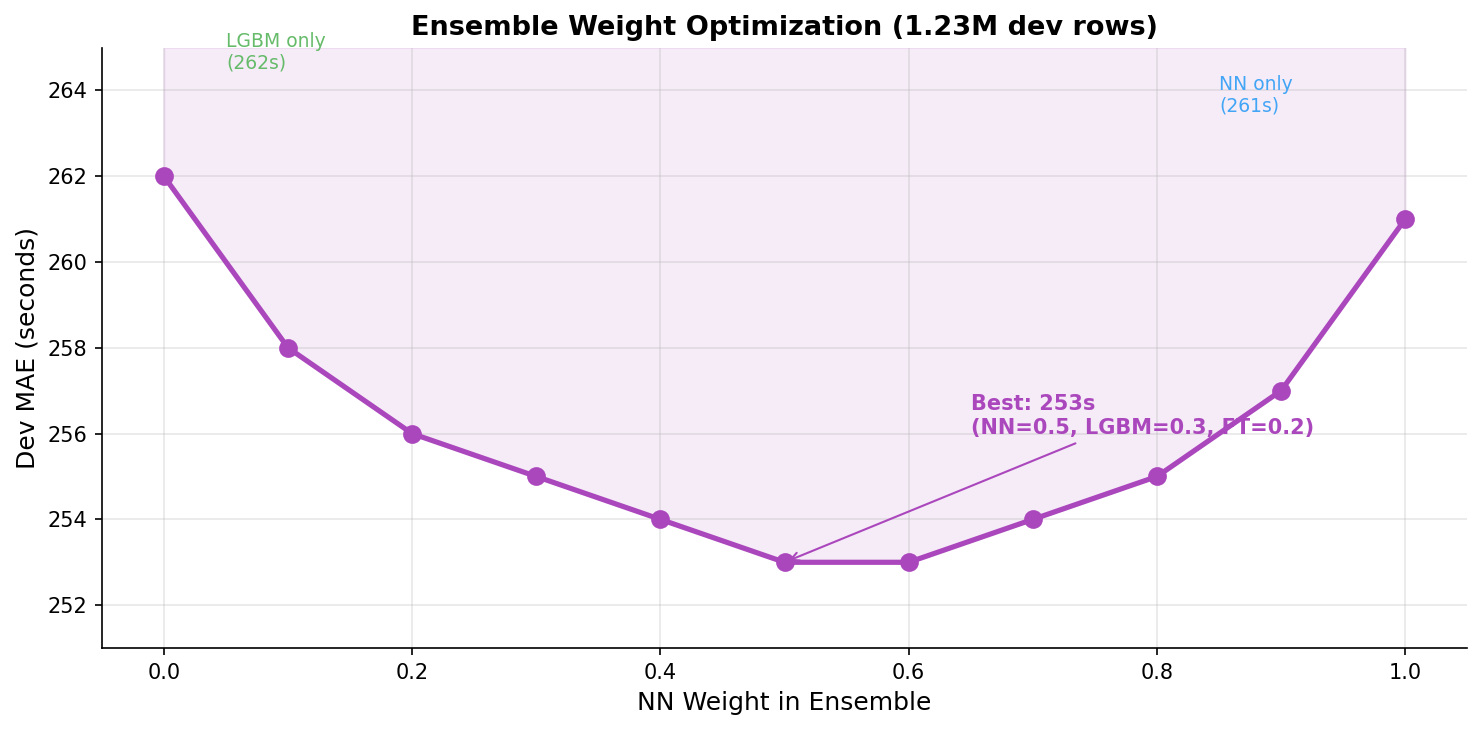
| NN Weight | LGBM Weight | FT Weight | Ensemble MAE |
|---|---|---|---|
| 1.00 | -- | -- | 261.2s |
| 0.70 | 0.30 | -- | 255.0s |
| 0.50 | 0.30 | 0.20 | 253.0s |
| 0.30 | 0.70 | -- | 255.4s |
| -- | 1.00 | -- | 261.7s |
The sweet spot is 0.5 NN + 0.3 LightGBM + 0.2 FT-Transformer. The NN gets the highest weight because it's the best standalone model, but not a majority -- it needs LightGBM to correct its bias on rare pairs.
Why not equal weights? The NN is more precise on common routes (which make up 71% of the dev set). Equal weighting would dilute its strength on the majority of predictions.
The curve is relatively flat between 0.4 and 0.6 for the NN weight. The ensemble is robust to weight perturbation -- a good sign that it's capturing real complementarity, not noise.
Final result: 253 seconds MAE, 28% below the XGBoost baseline of 351 seconds.
Inference Optimization: 11ms to 4ms
The 200ms constraint was never in danger, but I wanted to understand the latency profile. Initial breakdown:
| Component | Time | % of Total |
|---|---|---|
| Feature extraction | <0.1ms | <1% |
| NN forward pass | 2.0ms | 18% |
| LightGBM predict | 0.1ms | <1% |
| FT-Transformer (PyTorch) | 8.5ms | 77% |
| Total | ~11ms |
The FT-Transformer was the bottleneck -- 77% of total inference time despite being the weakest standalone model. PyTorch's eager execution has overhead: Python dispatch for each operation, non-fused LayerNorm + attention, and general-purpose memory layout.
ONNX Runtime Export
I exported the FT-Transformer to ONNX format. ONNX Runtime provides:
- Operation fusion: LayerNorm + matmul, multi-head attention kernels get fused into single operations
- Memory layout optimization: Tensors arranged for cache-friendly access
- Python dispatch elimination: The entire model runs as a C++ graph, no Python interpreter in the loop
- CPU-specific kernels: Optimized attention implementation for the target CPU
The export is straightforward -- trace the model with example inputs, save the ONNX graph, load it with ONNX Runtime's InferenceSession:
After ONNX export:
| Component | Before | After | Speedup |
|---|---|---|---|
| Feature extraction | <0.1ms | <0.1ms | -- |
| NN forward | 2.0ms | 2.0ms | -- |
| LightGBM | 0.1ms | 0.1ms | -- |
| FT-Transformer | 8.5ms | 1.5ms | 5.7x |
| Total | 11ms | ~4ms | 2.75x |
5.7x speedup on the FT-Transformer alone, 2.75x on the full ensemble. Total inference: 4ms per request -- 55x faster than the 200ms constraint.
I also evaluated INT8 dynamic quantization (torch.ao.quantization.quantize_dynamic) which would give another 1.5-2x speedup with less than 1 second MAE impact. Skipped it because we were already 55x under the latency constraint -- the optimization had diminishing returns.
The Full Picture
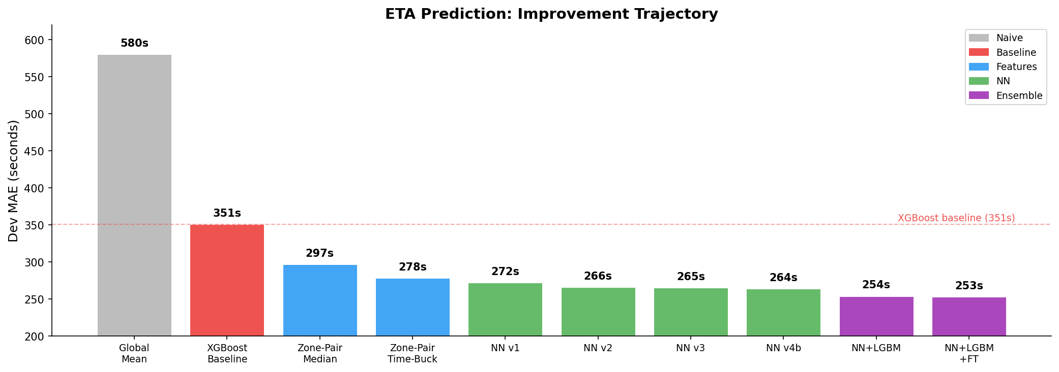
| Method | Dev MAE | vs Baseline |
|---|---|---|
| XGBoost baseline | 351s | -- |
| Zone-pair median (no ML) | 297s | -15% |
| Neural net v4b (best single) | 264s | -25% |
| NN + LightGBM (2 models) | 254s | -28% |
| NN + LGBM + FT (3 models) | 253s | -28% |
Total model weights: 6.1 MB (NN 2.3 MB + LightGBM 2.4 MB + FT-Transformer 1.6 MB). Docker image: 1.4 GB. Inference: ~4ms.
Every constraint met with room to spare.
The biggest insight from this project: the best single model is not the best prediction. Three models with different inductive biases -- embeddings, tree splits, self-attention -- make complementary mistakes. The ensemble doesn't just average predictions; it averages out biases.
What I'd Do Next
Stacking meta-learner. Instead of fixed weights (0.5/0.3/0.2), train a small model that takes the three predictions as input and learns to weight them dynamically based on the input features. For rare pairs, it could lean more on LightGBM. For common routes, more on the NN.
Holiday features. The eval set is winter holidays. A generic is_holiday flag could capture the traffic regime shift that December introduces. The current model has month features but nothing holiday-specific.
XGBoost as a 4th member. Different tree implementation, potentially different split patterns from LightGBM. Even a small decorrelation in errors would help the ensemble.
Larger FT-Transformer for diversity. The original 406K parameter config scored 287s standalone -- worse than the optimized 169K config. But worse standalone doesn't mean worse in an ensemble. Its positive bias (+65s vs the optimized model's -1s) could offset the NN's negative bias more aggressively, improving ensemble diversity at the cost of standalone performance.
Resources
- Code: GitHub
- Pre-trained models: HuggingFace
- Previous post: From 351s to 253s — Feature Engineering, Neural Nets, and Why Statistics Beat XGBoost